I calculated the invariant mass of dijets using the JetHT primary dataset in NanoAOD format from Run H of 2016 (/JetHT/Run2016H-UL2016_MiniAODv2_NanoAODv9-v1/NANOAOD). For this test, I worked with a single file:
root://eospublic.cern.ch//eos/opendata/cms/Run2016H/JetHT/NANOAOD/UL2016_MiniAODv2_NanoAODv9-v1/130000/0290F73B-A51C-A441-AEC1-8429F9CC8AA8.root
which I had already downloaded to my laptop before running the code.
#include “ROOT/RDataFrame.hxx”
#include “ROOT/RVec.hxx”
#include “TLorentzVector.h”
#include “TCanvas.h”
#include “TH1.h”
#include
#include
#include
using ROOT::RDataFrame;
using ROOT::RVec;
// — Helper: choose indices of the two best “good” jets (by pT)
static RVec SelectTop2GoodJets(const RVec& pt,
const RVec& eta,
const RVec& phi,
const RVec& mass,
const RVec& jetId)
{
RVec good;
good.reserve(pt.size());
// Quality & kinematics (2016 UL): pT>30 GeV, |eta|<2.4, Tight ID (bit 1 → value 2)
for (int i = 0; i < (int)pt.size(); ++i) {
const bool kinOK = (pt[i] > 30.f) && (std::abs(eta[i]) < 2.4f);
const bool idOK = (jetId[i] & 2); // Tight
if (kinOK && idOK) good.push_back(i);
}
if (good.size() < 2) return {};
std::sort(good.begin(), good.end(), [&](int a, int b){ return pt[a] > pt[b]; });
return RVec{ good[0], good[1] };
}
// — Helper: compute Mjj from selected jet indices
static double ComputeMjj(const RVec& pt,
const RVec& eta,
const RVec& phi,
const RVec& mass,
const RVec& idx)
{
if (idx.size() < 2) return -1.0;
TLorentzVector j1, j2;
j1.SetPtEtaPhiM(pt[idx[0]], eta[idx[0]], phi[idx[0]], mass[idx[0]]);
j2.SetPtEtaPhiM(pt[idx[1]], eta[idx[1]], phi[idx[1]], mass[idx[1]]);
return (j1 + j2).M();
}
// — Main macro
void dijetsmjjonly()
{
const std::string file =
“root://eospublic.cern.ch//eos/opendata/cms/Run2016H/JetHT/NANOAOD/UL2016_MiniAODv2_NanoAODv9-v1/130000/0290F73B-A51C-A441-AEC1-8429F9CC8AA8.root”;
ROOT::EnableImplicitMT();
// Build dataframe
RDataFrame df(“Events”, file);
// Select two jets and compute Mjj
auto df2 = df
.Define(“TwoJetsIdx”, SelectTop2GoodJets,
{“Jet_pt”,“Jet_eta”,“Jet_phi”,“Jet_mass”,“Jet_jetId”})
.Filter(“TwoJetsIdx.size() == 2”, “Need >= 2 good jets”)
.Define(“Mjj”, ComputeMjj,
{“Jet_pt”,“Jet_eta”,“Jet_phi”,“Jet_mass”,“TwoJetsIdx”});
// Book the Mjj histogram (adjust range/binning as you like)
auto hMjj = df2.Histo1D(
{“hMjj”,“Dijet invariant mass;M_{jj} [GeV];Events”, 120, 0., 3000.},
“Mjj”);
// Draw
TCanvas c(“c”,“Mjj”,1000,800);
//gPad->SetLogy(); // Log-y is often useful for wide mass spectra
hMjj->SetLineWidth(2);
hMjj->Draw();
c.Update();
c.SaveAs(“Mjj.png”);
//c.SaveAs(“Mjj.pdf”);
}
end of my code
The resulting plot from executing this code is presented here:
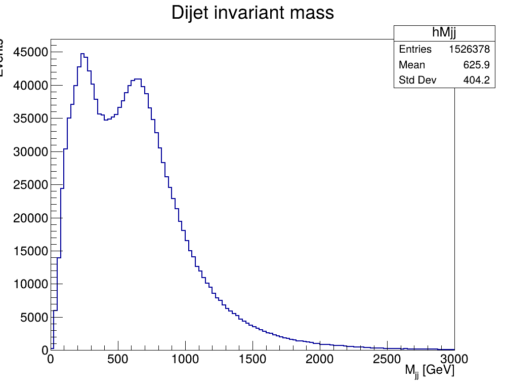
I would like to ask whether the appearance of the second peak is a normal or expected feature when analyzing data collected with high-threshold triggers, such as the dataset I am using, or if it indicates that something is missing in my code or that my implementation is incorrect.